
R Markdown, Jekyll, and Footnotes
8 minute read
Update: 05/19/2021 John MacFarlane helpfully pointed out that this is all incredibly unnecessary because pandoc makes it easy to add support for footnotes to GitHub-Flavored Markdown. The documentation notes that you can add extensions to output formats they don’t normally support. Since standard markdown natively supports footnotes when used as an output format, I didn’t even think to look into manually enabling them for GitHub-Flavored Markdown.
If you’re running pandoc from the command line all you need to do is add -t gfm+footnotes to your pandoc command. If you’re working with .Rmd files like me, all you need to do is add +footnotes to the end of of the variant: gfm line in your YAML header. As a side benefit, you can drop the --wrap=preserve flag and end up with .md files that aren’t hundreds of columns wide. I’m leaving the original post up below in case anyone who has an even weirder use case than me might find it helpful, or if any of my students ever stumble across this page and don’t believe that I’m still constantly learning, too.
I use jekyll to create my website. Jekyll converts Markdown files into the HTML that your browser renders into the pages you see. As others and I have written before, it’s pretty easy to use R Markdown to generate pages with R code and output all together. One thing has consistently eluded me, however: footnotes.
Every time I try to include footnotes in my .Rmd file, they end up mangled and not actually footnotes in the final HTML page. My solution thus far has been to just avoid footnotes and lean heavily on parenthetical asides when I’m using R Markdown to generate a page. My recent post on using SQL style filtering to preprocess large spatial datasets before loading them into memory needed a whopping six footnotes, so I finally had to sit down and figure it out.
What’s happening
The ‘standard’ method for adding footnotes in R Markdown is actually a bit of a cheat compared to the method in the official Markdown specification. R Markdown lets you use a LaTeX-esque syntax for defining footnotes:
Here is some body text.^[This footnote will appear at the bottom of the page.]
However, Jekyll uses the official Markdown specification for footnotes, so this won’t work. Instead, we need to define them with the official syntax:
Here is some body text.[^1]

[^1]: This footnote will appear at the bottom of the page.
However, when R Markdown converts your file from standard Markdown to GitHub-Flavored Markdown, something strange happens and the output in your .md file will look like this:
Here is some body text.\[1\]

1. This footnote will appear at the bottom of the page.
When Jekyll converts the Markdown file to HTML, you end up with a sad lonely unclickable [1] where your footnote should go. The content of the footnote does appear at the bottom of the page, but it lacks the footnote formatting so it just looks like regular text and there’s no link to click and return to the footnote’s place in the text.
Why it’s happening
Understanding what’s happening here (and thus how to fix it) requires a slightly detailed explanation of what exactly happens when you hit that Knit button in RStudio. First, the knitr package runs all of the code in your .Rmd file and creates a .md file. Next, pandoc takes the .md file and converts it to whatever output format you want.1

Pandoc is the source of our problems here. The square braces that set off a footnote are metacharacters in Markdown, since they’re used to construct links (among other things, like citations with pandoc-citeproc). When Pandoc sees them in the process of converting from standard Markdown to GitHub-Flavored Markdown, it (logically) decides that they’re important content and preserves them by escaping them with a backslash so they’re preserved in the GitHub-Flavored Markdown. Unfortunately for us, we want our square brackets to be treated as special characters and not turned into text. This is a known issue with Pandoc (see this issue on GitHub) so it will eventually get fixed, but in the meantime I’ve come up with a workaround.
How to fix it
Pandoc allows you to tag both code chunks and inline code with a special raw attribute which will ensure they’re passed on to the output format unmodified. To do this, just enclose any text with backticks (`) and then put {=markdown} immediately after the closing backtick. This will ensure that Pandoc doesn’t alter the ‘code’ in the backticks at all. It’s debatable whether the [^1] used to define a footnote is really code, but for our purposes treating it like code will ensure that our footnotes work in the final output:
Here is some body text.`[^1]`{=markdown}

`[^1]:`{=markdown} This footnote will appear at the bottom of the page.
There’s one more tweak we have to make to get this to work. If any of your footnotes are longer than 72 characters,2 then Pandoc will split them up and divide them into multiple lines in the output .md file. Since footnotes need to be all on the same line, this will break them and you’ll have a bunch of sentence fragments at the end of your page right above the equally fragmented footnotes. To fix this, we need to use the --wrap argument to Pandoc in our YAML header. Below is the YAML header for the .Rmd file that generates the .md file that Jekyll uses to generate the HTML your browser uses to render this page.
---
title: Footnotes in `.Rmd` files
output:
  md_document:
    variant: gfm
    preserve_yaml: TRUE
    pandoc_args:
      - "--wrap=preserve"
knit: (function(inputFile, encoding) {
  rmarkdown::render(inputFile, encoding = encoding, output_dir = "../_posts") })
date: 2020-10-26
permalink: /posts/2020/10/jeykll-footnotes
excerpt_separator: <!--more-->
toc: true
tags:
  - jekyll
  - rmarkdown
---
By specifying --wrap=preserve, we tell Pandoc to respect the line breaks present in the .Rmd file when generating the .md file.3 Accordingly, our footnotes will be intact and functional in the final web page.
Proof
And now, to prove to you that this post really did start out as a .Rmd file, here’s some R code and a plot. Everyone’s seen mtcars a million times, and it turns out that iris was originally published in the Annals of Eugenics, so I went digging for a new built in dataset.4 I landed on the Loblolly pines dataset, which records the height of 14 different loblolly pine trees.5
library(ggplot2)
ggplot(Loblolly, aes(x = age, y = height, group = Seed)) +
  geom_line(alpha = .5) +
  labs(x = 'Age (years)', y = 'Height (feet)') +
  theme_bw()
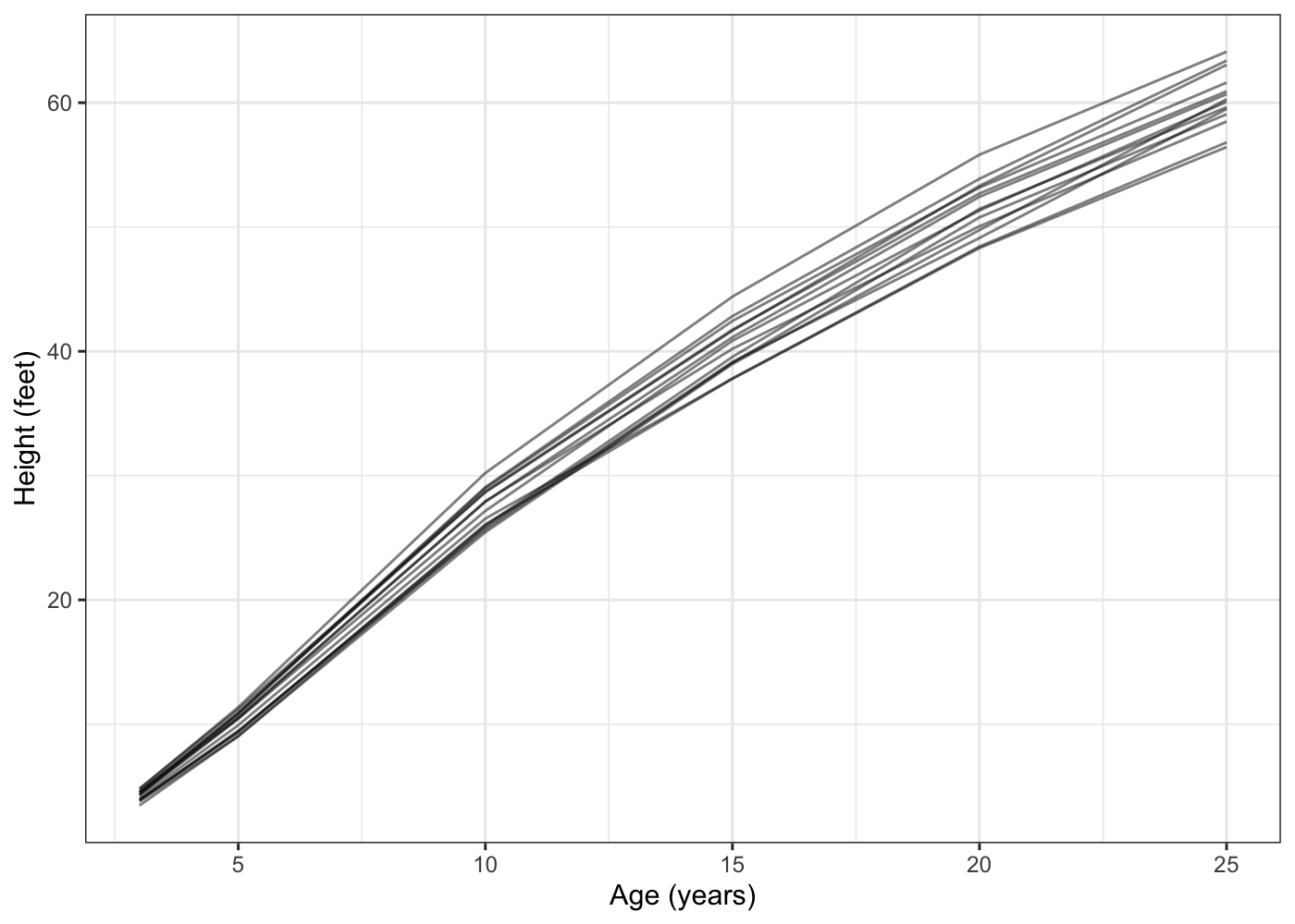
It looks like all of the trees in the sample followed a pretty similar growth trajectory! Finally, to really really prove this page started out as a .Rmd file, here’s the sessionInfo():
sessionInfo()
## R version 4.0.2 (2020-06-22)
## Platform: x86_64-apple-darwin17.7.0 (64-bit)
## Running under: macOS High Sierra 10.13.6
##
## Matrix products: default
## BLAS:   /System/Library/Frameworks/Accelerate.framework/Versions/A/Frameworks/vecLib.framework/Versions/A/libBLAS.dylib
## LAPACK: /System/Library/Frameworks/Accelerate.framework/Versions/A/Frameworks/vecLib.framework/Versions/A/libLAPACK.dylib
##
## locale:
## [1] en_US.UTF-8/en_US.UTF-8/en_US.UTF-8/C/en_US.UTF-8/en_US.UTF-8
##
## attached base packages:
## [1] stats     graphics  grDevices utils     datasets  methods   base
##
## other attached packages:
## [1] ggplot2_3.3.2
##
## loaded via a namespace (and not attached):
##  [1] rstudioapi_0.11      knitr_1.30           magrittr_1.5
##  [4] tidyselect_1.1.0     munsell_0.5.0        colorspace_1.4-1
##  [7] here_0.1             R6_2.4.1             rlang_0.4.8
## [10] dplyr_1.0.2          stringr_1.4.0        tools_4.0.2
## [13] grid_4.0.2           gtable_0.3.0         xfun_0.18
## [16] withr_2.3.0          htmltools_0.5.0.9001 ellipsis_0.3.1
## [19] yaml_2.2.1           rprojroot_1.3-2      digest_0.6.25
## [22] tibble_3.0.4         lifecycle_0.2.0      crayon_1.3.4
## [25] purrr_0.3.4          vctrs_0.3.4          glue_1.4.2
## [28] evaluate_0.14        rmarkdown_2.3        stringi_1.5.3
## [31] compiler_4.0.2       pillar_1.4.6         generics_0.0.2
## [34] scales_1.1.1         backports_1.1.10     pkgconfig_2.0.3
Pandoc is incredibly powerful, but it’s also incredibly opaque and difficult to learn. You can create incredibly fancy PDF and HTML documents in R Markdown without ever having to know anything about Pandoc. ↩
The default output width defined by the
--columnsargument to Pandoc. ↩You can also use
--wrap=none, which will put every paragraph in a single gigantic line of text. ↩If you’re willing to install additional packages, Allison Horst’s palmerpenguins package is fantastic and fills much the same educational niche as
iris. See here for even more alternatives. ↩Fun fact, loblolly pine seeds were carried aboard Apollo 14 and subsequently planted throughout the US. ↩