
Working with Large Spatial Data in R
22 minute read
In my research I frequently work with large datasets. Sometimes that means datasets that cover the entire globe, and other times it means working with lots of micro-level event data. Usually, my computer is powerful enough to load and manipulate all of the data in R without issue. When my computer’s fallen short of the task at hand, my solution has often been to throw it at a high performance computing cluster. However, I finally ran into a situation where the data proved too large even for that approach.
As a result, I finally had to teach myself how to break large spatial datasets into more manageable chunks. In the process a learned a little SQL and a lot about the underlying software libraries that power the r-spatial ecosystem of R packages. In this post, I walk through the workflow I developed for this task and explain the logic behind each step.
On disk
The general idea is to work with data ‘on disk’ instead of ‘in memory’. Normally, when you load a dataset into R, your computer reads it from whatever storage media it uses (hard drive or solid state drive) into memory (RAM). Memory is considerably faster to read from and write to than storage, which is what lets you complete simple operations in R in the blink of an eye. Most consumer computers have much more storage than RAM (my 2015 MacBook Pro has 256 GB of storage and 8 GB of memory) so it’s very possible to end up with a dataset larger than your computer’s memory. In fact, it doesn’t have to be anywhere near the size of your computer’s memory to bump into this limit because every other application you have running uses up memory as well.
To deal with this issue, you can extract just the parts of a dataset you need to work with at any given time; this subset will be loaded into memory, and the rest remain on disk and invisible to R1. There are a couple of R packages that exist for dealing with this issue, such as bigmemory for basic R data types like numerics or disk.frame for dplyr-compatible operations, but neither supports spatial data.
I’m going to use the cshapes to illustrate and explain this workflow2. You can download and extract it from within R:
## download cshapes dataset
download.file('http://downloads.weidmann.ws/cshapes/Shapefiles/cshapes_0.6.zip',
              'cshapes.zip')

## extract cshapes dataset
unzip('cshapes.zip')

## check that dataset extracted correctly
list.files(path = '.', pattern = 'cshapes')
## [1] "cshapes_shapefile_documentation.txt" "cshapes.dbf"
## [3] "cshapes.prj"                         "cshapes.shp"
## [5] "cshapes.shx"                         "cshapes.zip"
Then use the sf package to load the data and check them out:
## load packages
library(tidyverse)
library(sf)

## read in cshapes
cshapes <- st_read('cshapes.shp')
The cshapes dataset is specifically designed to be easy to load and manipulate on a conventional laptop computer. To do this, it sacrifices a significant degree of detail in the polygons that represent each individual state. For many analyses, this is fine and won’t affect the results. However, sometimes you need to measure the length of borders between states, and the coastline paradox dictates that you use the most high resolution spatial data possible. In that case, the data might be too large for your computer to hold in memory. If that’s the case, then it’s time to start thinking about leaving the data on disk and only loading what you really need at any given point.
SQL
Luckily the sf package supports SQL queries to filter the data on disk and only read in a subset of the total data. SQL is a language for interacting with relational databases, and is incredibly fast compared to loading data into R and then filtering it. SQL has many variants, referred to as dialects, and the sf package uses one called OGR SQL dialect to interact with spatial datasets. The basic structure of a SQL call is SELECT col FROM "table" WHERE cond.
SELECTtells the database what columns (fields in SQL parlance) we wantFROMtells the database what table (databases can have many tables) to select those columns fromWHEREtells that database we only want rows where some condition is true
If you use the tidyverse a lot, this may seem familiar to you because it’s pretty similar to dplyr syntax, except dplyr already knows which data frame you want to work with. If we want to only load one polygon at a time into R, then we need to know the field (or combination of fields) that uniquely identifies a polygon. To demonstrate, let’s load just the polygon for Morocco that begins in 1976 when it annexed the Northern part of Western Sahara. Let’s cheat by looking at the data I’ve loaded into R:
## filter to Morocco beginning in 1976
cshapes %>% filter(CNTRY_NAME == 'Morocco', GWSYEAR == 1976)
## Simple feature collection with 1 feature and 24 fields
## geometry type:  MULTIPOLYGON
## dimension:      XY
## bbox:           xmin: -15.22687 ymin: 23.11465 xmax: -1.011809 ymax: 35.91916
## geographic CRS: WGS 84
##   CNTRY_NAME     AREA CAPNAME CAPLONG CAPLAT FEATUREID COWCODE COWSYEAR COWSMONTH COWSDAY COWEYEAR
## 1    Morocco 576351.8   Rabat   -6.83  34.02       220     600     1976         4       1     1979
##   COWEMONTH COWEDAY GWCODE GWSYEAR GWSMONTH GWSDAY GWEYEAR GWEMONTH GWEDAY ISONAME ISO1NUM ISO1AL2
## 1         8       4    600    1976        4      1    1979        8      4 Morocco     504      MA
##   ISO1AL3                       geometry
## 1     MAR MULTIPOLYGON (((-4.420418 3...
The cshapes dataset records when states change territorial boundaries or capital locations, so the combination of a state name or identifier and a start or end date uniquely identifies all rows in the data. Since, this polygon begins on April 1, 1976 and the Gleditsch and Ward code for Morocco is 600, plugging it all into the query argument to st_read() gets us:
## read in morocco polygon
morocco <- st_read('cshapes.shp',
                   query = 'SELECT * FROM "cshapes" WHERE GWCODE = 600 AND GWSYEAR = 1976 AND GWSMONTH = 4 AND GWSDAY = 1')

## verify country name
morocco$CNTRY_NAME
## [1] "Morocco"
Awesome! We were able to read in just one polygon from the cshapes dataset. Note that * means all columns. As I mentioned above, this is cheating, since we had to read the whole dataset into R with a standard st_read() call to learn the names and values of the variables we then filtered on.
Sneaking a peek
When this isn’t an option, we can sneak a peak at the data by loading just the first observation into R. This requires significantly less memory than loading an entire dataset, and can give us the information we need to filter the full dataset and read in one observation at a time. Most SQL implementations don’t have row numbers, so it’s hard to just grab the first row of the data for this purpose. However, the OGR SQL dialect documentation notes that it implements a special field called FID that is a feature ID, i.e., a row number. We can take advantage of FID to select the first polygon from the data using the query argument to st_read() again:
## read in first row of the data
cshapes_row <- st_read('cshapes.shp', query = 'SELECT * FROM "cshapes" WHERE FID = 1')

## inspect
cshapes_row
## Simple feature collection with 1 feature and 24 fields
## geometry type:  POLYGON
## dimension:      XY
## bbox:           xmin: -58.0714 ymin: 1.836245 xmax: -53.98612 ymax: 6.001809
## geographic CRS: WGS 84
##   CNTRY_NAME     AREA    CAPNAME CAPLONG   CAPLAT FEATUREID COWCODE COWSYEAR COWSMONTH COWSDAY
## 1   Suriname 145952.3 Paramaribo   -55.2 5.833333         1     115     1975        11      25
##   COWEYEAR COWEMONTH COWEDAY GWCODE GWSYEAR GWSMONTH GWSDAY GWEYEAR GWEMONTH GWEDAY  ISONAME
## 1     2016         6      30    115    1975       11     25    2016        6     30 Suriname
##   ISO1NUM ISO1AL2 ISO1AL3                 _ogr_geometry_
## 1     740      SR     SUR POLYGON ((-55.12796 5.82217...
Even if we knew that the data had an ID column and start and end dates, we wouldn’t know the precise formatting (capitalization, underscores or dashes) of column names, or whether start and end dates are stored as one column or sets of three like they are here.
Making a list
We still need more information if we want to iterate through the polygons in the data and load them one at a time. We know what columns uniquely identify the rows, but what don’t know all the values they take on. Without that, we we’re stuck. What (usually) makes spatial data big is not the tabular data themselves, but the spatial features they’re attached to. This is particularly the case with polygons, which can be incredibly large in size for complex features. So, the goal here is to get the data we care about (ID column and start date) and ditch everything else, loading only the bare minimum into memory.
To do this, we’ll use the ogr2ogr() function in the gdalUtils package3. ogr2ogr() converts between different spatial data formats. It also offers two features that we’re going to use to cut down the data to the bare minimum. The select argument is a SQL selection, so we’re going to create a comma separated list of our key columns. The nlt argument specifies what type of geometry to create in the output. Conveniently it accepts NONE as a value, which will yield a plain table of data with none of the memory-hogging geometries:
## load package
library(gdalUtils)

## convert to nonspatial geometry
ogr2ogr(src_datasource_name = 'cshapes.shp', dst_datasource_name = 'cshapes_no_geom',
        select = 'GWCODE,GWSYEAR,GWSMONTH,GWSDAY', nlt = 'NONE')
This will create a shapefile in the new directory cshapes_no_geom called cshapes. The usual .shp and .shx components of a shapefile are missing, but the .dbf part is there, and that’s the one we care about. Load it up with st_read() and we’ll have what we need:
## load non-geometry table
cshapes_id <- st_read('cshapes_no_geom/cshapes.dbf')

## inspect
head(cshapes_id)
##   GWCODE GWSYEAR GWSMONTH GWSDAY
## 1    110    1966        5     26
## 2    115    1975       11     25
## 3     52    1962        8     31
## 4    101    1946        1      1
## 5    990    1962        1      1
## 6    972    1970        6      4
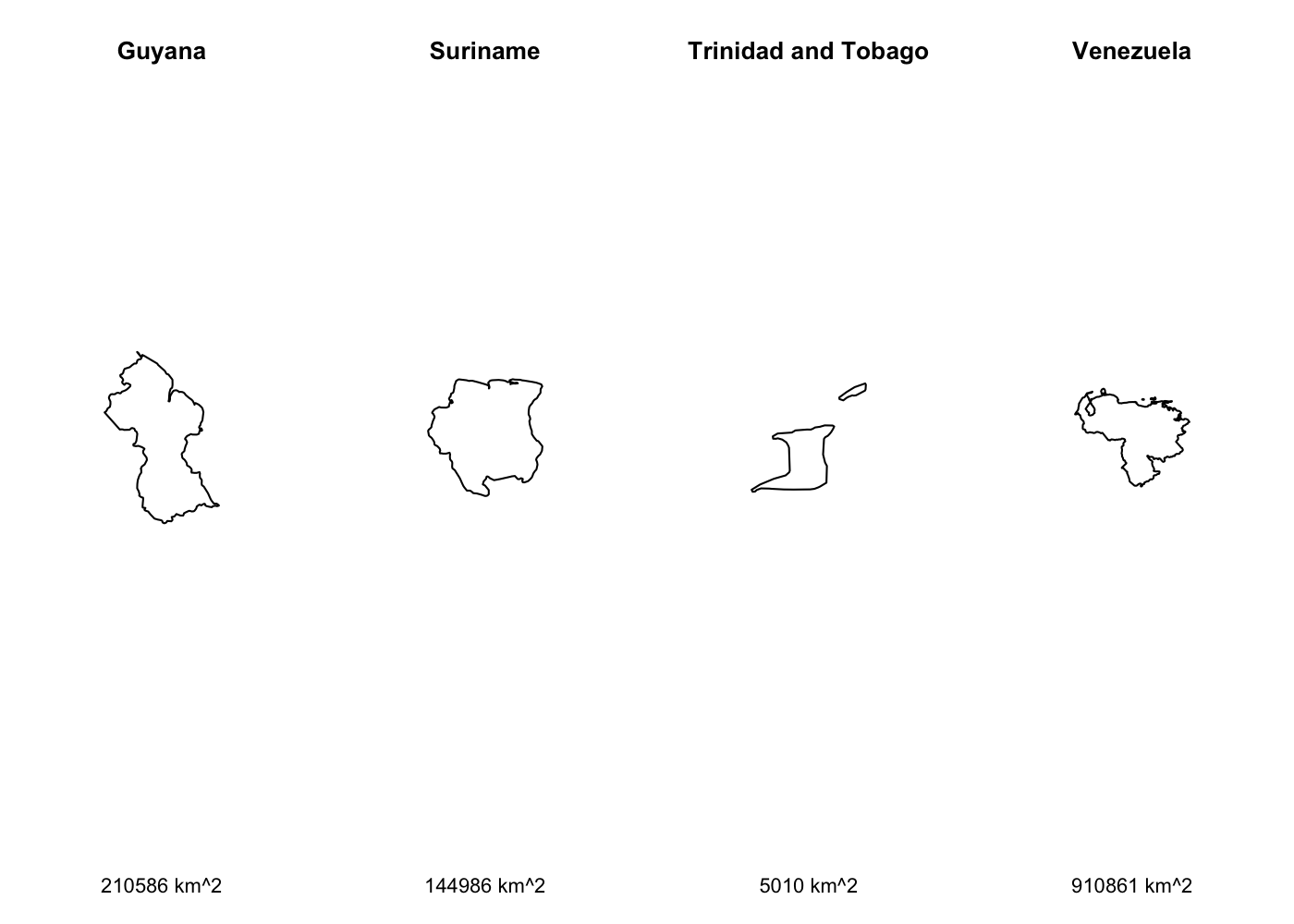
Now you can load polygons one at a time and perform whatever geometric operations you need to. To illustrate, I’ll load the first four polygons in the dataset, calculate their area, and then plot them.
## set up four panel plot
par(mfrow = c(1, 4), mar = c(6.1, 4.1, 4.1, 4.1))

## read in each polygon and plot
for (i in 1:4) {

  ## build SQL query
  query_str <- str_c('SELECT * FROM "cshapes" WHERE GWCODE = ', cshapes_id$GWCODE[i],
                     ' AND GWSYEAR = ', cshapes_id$GWSYEAR[i],
                     ' AND GWSMONTH = ', cshapes_id$GWSMONTH[i],
                     ' AND GWSDAY = ', cshapes_id$GWSDAY[i])

  ## read in data
  pol <- st_read('cshapes.shp', query = query_str)

  ## plot data
  pol %>%
    st_geometry() %>%
    plot(main = pol$CNTRY_NAME,
         sub = str_c(round(units::set_units(st_area(pol), 'km^2'), digits = 0),
                      ' km^2'))

}
Won’t you be my neighbor?
Sometimes (oftentimes in spatial analysis) we need not just a polygon, but also its neighbors. That means loading just one polygon is insufficient. If your data are already in R, this is easy with the st_filter() function, but it’s much trickier if you’re trying to filter data before loading them into R4. Luckily, st_read() as you covered! The wkt_filter accepts a well-known text string that can be used to filter the data before loading them into R5. Well-known text is a standard string representation of geometry, and is actually how the sf package prints geometry in R:
st_point(c(1, 2))
We want to use the wkt_filter argument to only load polygons that intersect with our Morocco polygon into R. To do that, we need to convert our polygon to a well-known text string with the st_as_text() function, then pass it to st_read(). However, st_as_text() only accepts sfc and sfg objects, not sf objects:
## create well known text object to filter cshapes on disk
morocco_wkt <- st_as_text(morocco)
## Error in UseMethod("st_as_text"): no applicable method for 'st_as_text' applied to an object of class "c('sf', 'data.frame')"
To get around this, we need to drop the data on morocco and extract just the geometry of the polygon with st_geometry():
## create well known text object to filter cshapes on disk
morocco_wkt <- morocco %>%
  st_geometry() %>% # convert to sfc
  st_as_text() # convert to well known text

## plot morocco and neighbors
st_read('cshapes.shp', wkt_filter = morocco_wkt) %>%
  st_geometry() %>%
  plot(main = morocco$CNTRY_NAME)

## add morocco polygon on top
morocco %>%
  st_geometry() %>%
  plot(add = T, col = rgb(0, 1, 0, .5))
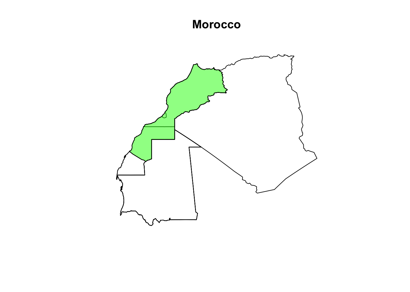
Notice that there are multiple polygon boundaries within the green area of our green Morocco polygon. That’s because there are 4 Morocco polygons in the data starting in 1956, 1958, 1976, and 1979. Be sure to filter the dataset, either as part of the SQL query or in a dplyr::filter() so that you only get polygons that existed contemporaneously with your polygon of interest.
Wrapping up
So far, we’ve covered:
- How to extract the first polygon for a spatial dataset and learn the names of identifier columns
- How to strip the geometry from a spatial dataset and extract just a table of these columns
- How to use these columns to iterate through the polygons in the dataset and import them one at a time, or along with their neighbors
You can technically skip the first two steps and just move the .shp and .shx files out of the directory before loading the .dbf file with st_read(), but that kind of feels like cheating to me6 and it only works with shapefiles. If you have another type of spatial dataset, read on.
This time for real
In my research, I often need to work with spatial data that’s measured at or aggregated up to different administrative divisions (ADMs). GADM helpfully provides a global dataset of ADMs. Although you can download ADMs for specific countries, I work with data in enough different countries that I finally decided to just download the entire dataset. While the cshapes example above just illustrated how to implement a pipeline for working with spatial data on disk, you may actually need to use one with these data depending on your machine’s hardware.
This master dataset comes as a GeoPackage. Most importantly for us, that means we can’t just delete a few component files to load the non-spatial table from the dataset; we have to convert it from a spatial dataset to a non-spatial one with ogr2ogr(). The GeoPackage contains ADMs from level 0 (countries) all the way down to level 5. Each level is stored as a separate layer in the .gpkg, and we can get a list of available layers with the st_layers() function:
## get layers
st_layers('~/Dropbox/Datasets/GADM/gadm34_levels_gpkg/gadm34_levels.gpkg')
## Driver: GPKG
## Available layers:
##   layer_name geometry_type features fields
## 1     level0 Multi Polygon      256      2
## 2     level1 Multi Polygon     3610     10
## 3     level2 Multi Polygon    45962     13
## 4     level3 Multi Polygon   147427     16
## 5     level4 Multi Polygon   138053     14
## 6     level5 Multi Polygon    51427     15
We want to work with the third-order administrative divisions (cities, towns, and other municipalities in the US context), so we need the level3 layer. Where we just used the name of the dataset in our SQL call before, this time we’ll use level3. Now we just follow the same workflow as with the cshapes dataset above:
## get first observation
level3 <- st_read('~/Dropbox/Datasets/GADM/gadm34_levels_gpkg/gadm34_levels.gpkg',
                  query = 'SELECT * FROM "level3" WHERE FID = 1', layer = 'level3')

## inspect
level3
## Simple feature collection with 1 feature and 16 fields
## geometry type:  MULTIPOLYGON
## dimension:      XY
## bbox:           xmin: 13.08792 ymin: -8.010127 xmax: 13.59943 ymax: -7.708598
## geographic CRS: WGS 84
##   GID_0 NAME_0   GID_1 NAME_1 NL_NAME_1     GID_2 NAME_2 NL_NAME_2       GID_3 NAME_3 VARNAME_3
## 1   AGO Angola AGO.1_1  Bengo      <NA> AGO.1.1_1 Ambriz      <NA> AGO.1.1.1_1 Ambriz      <NA>
##   NL_NAME_3  TYPE_3 ENGTYPE_3 CC_3 HASC_3                           geom
## 1      <NA> Commune   Commune <NA>   <NA> MULTIPOLYGON (((13.12764 -7...
This time we have a single column that uniquely identifies observations, GID_3, so we only have to extract one column from the dataset. We use the ogr2ogr() function as before, but we have to specify the layer = 'level3' argument since the GeoPackage has more than one layer and we want to work with a specific one. Since GID_3 is our identifier column, that’s what we select from the dataset:
## convert to nonspatial geometry
ogr2ogr(src_datasource_name = '/Users/Rob/Dropbox/Datasets/GADM/gadm34_levels_gpkg/gadm34_levels.gpkg',
        dst_datasource_name = 'gadm34_levels_no_geom',
        layer = 'level3',
        select = 'GID_3',
        nlt = 'NONE')

## load non-geometry table
gadm_ids <- st_read('gadm34_levels_no_geom/level3.dbf')

## inspect
head(gadm_ids)
##         GID_3
## 1 AGO.1.1.1_1
## 2 AGO.1.1.2_1
## 3 AGO.1.1.3_1
## 4 AGO.1.2.1_1
## 5 AGO.1.2.2_1
## 6 AGO.1.2.3_1
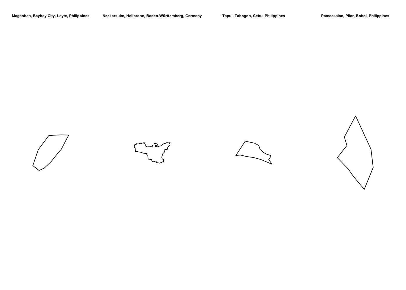
And we can again read the polygons into R one at a time and perform whatever spatial operations we need. Since our identifying column is a string this time, we need to enclose it quotes in our SQL call. SQL is very picky about quotation mark types, so while we needed to surround our layer name with double quotes, we need to surround our identifier variable with single quotes. I’m already using single quotes to define the character string for the SQL call, so I need to escape the single quotes around the identifier. You can do this with a single backslash (\). Thus, you can include single quotes in a single-quoted string like this: 'this is a string \'this is another part of a string\''. Other than that wrinkle, things are pretty much the same as with cshapes:
## for reproducibility
set.seed(27599)

## set up four panel plot
par(mfrow = c(1, 4), mar = c(2.1, 4.1, 4.1, 4.1))

## read in each polygon and plot
for (i in sample(1:nrow(gadm_ids), 4, replace = F)) { # mix it up

  ## build SQL query
  query_str <- str_c('SELECT * FROM "level3" WHERE GID_3 = \'',
                     gadm_ids$GID_3[i], '\'')

  ## read in polygon for ADM3 i
  adm3 <- st_read('~/Dropbox/Datasets/GADM/gadm34_levels_gpkg/gadm34_levels.gpkg',
                  query = query_str, layer = 'level3')

  ## plot polygon and label with full name
  print(plot(adm3$geom,
             main = adm3 %>%
               select(starts_with('NAME_')) %>% # get all name variables
               st_drop_geometry() %>% # drop geometry
               rev() %>% # reverse order of names to 3, 2, 1, 0
               str_c(collapse = ', '), # collapse w/ commas
             cex.main = .6))

}
 Spatially filtering the GADM dataset is just as easy as with cshapes. To illustrate, I’m going to pull out a random polygon and use it to filter the data. However, these are third-order administrative divisions, and so it’s possible that even capturing all adjacent polygons won’t cover a very large area. To deal with this concern, we can buffer the polygon with the
 st_buffer() function before we convert it to well-known text:
## import single polygon
adm3 <- st_read('~/Dropbox/Datasets/GADM/gadm34_levels_gpkg/gadm34_levels.gpkg',
                  query = str_c('SELECT * FROM "level3" WHERE FID = 63130'))

## create well known text object to filter GADM on disk
adm3_wkt <- adm3 %>%
  st_geometry() %>% # convert to sfc
  st_buffer(.025) %>% # buffer .05 decimal degrees
  st_as_text() # convert to well known text

## plot Dakkoun and neighbors w/in .05 decimal degrees
st_read('~/Dropbox/Datasets/GADM/gadm34_levels_gpkg/gadm34_levels.gpkg',
        layer = 'level3', wkt_filter = adm3_wkt) %>%
  st_geometry() %>%
  plot(main = adm3 %>%
               select(starts_with('NAME_')) %>%
               st_drop_geometry() %>%
               rev() %>%
               str_c(collapse = ', '))

## plot Dakkoun and highlight
adm3 %>%
  st_geometry() %>%
  plot(add = T, col = 'green')

## plot buffered polygon used to filter GADM on disk
adm3 %>%
  st_geometry() %>%
  st_buffer(.025) %>%
  st_cast('LINESTRING') %>%
  plot(add = T, col = 'blue')
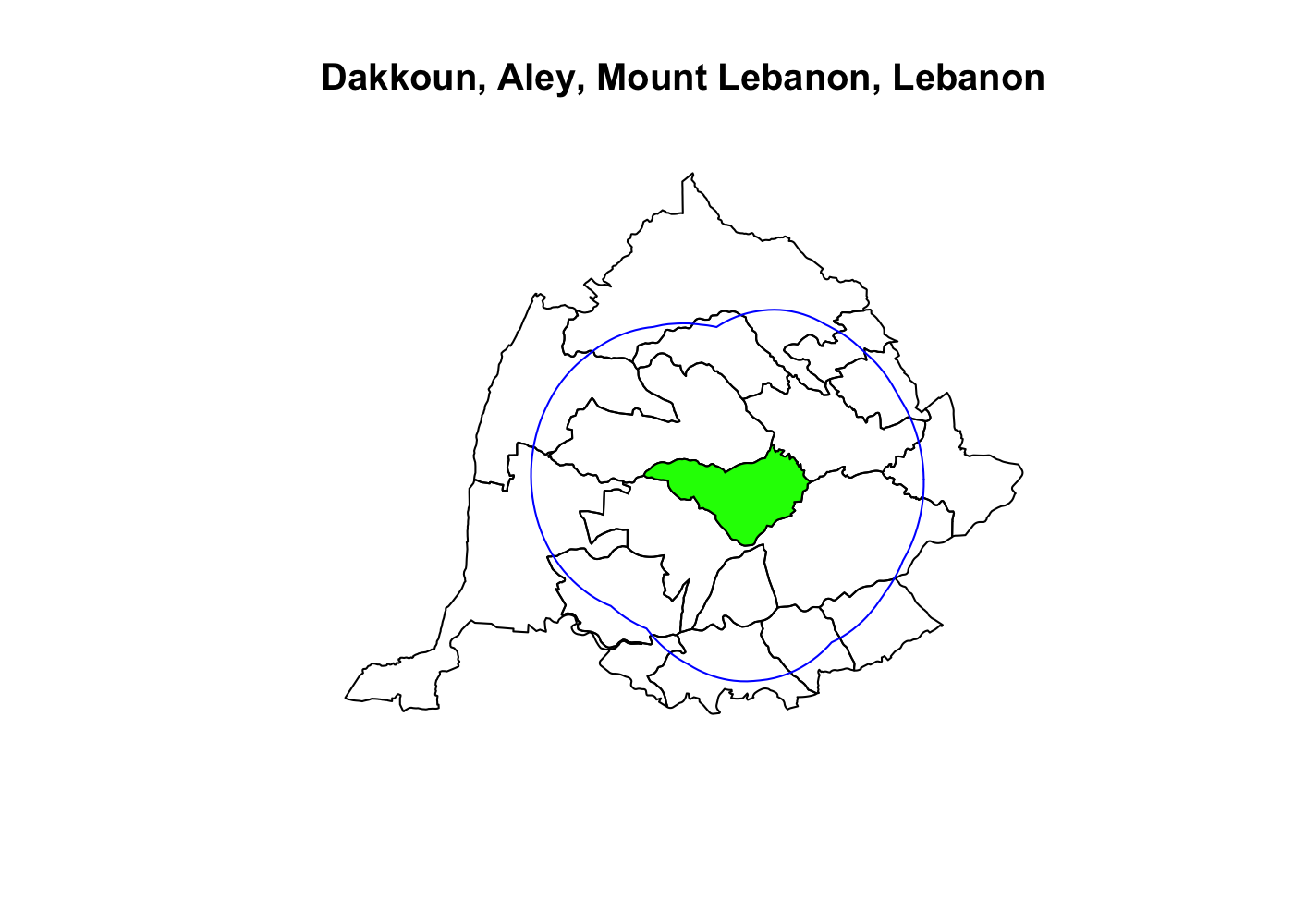
The green polygon above is Dakkoun, the 63,130th polygon in the the dataset. The blue line is the extent of the .025 decimal degree buffer applied to it to before filtering the dataset. This workflow can speed things up when working with these data, considering there are 884,562 third-order administrative division polygons in the dataset.
Making data manageable
The query and wkt_filter arguments to st_read() can help you work with large spatial datasets that are either too big to load into memory, or too slow to work with once loaded. While this is less of a concern with low resolution datasets created by social scientists, it can be incredibly useful if you ever have to work with super high resolution data created by remote sensing technologies or actual cartographers and geographers.
This is the appraoch that the raster package uses. R only stores information on the extent and resolution of a raster in memory; the actual values in each cell of a raster are only loaded into memory when accessed by R using a function like
extract(). ↩Although I’m using cshapes as an example throughout this post so you can easily follow along and run the code yourself, it’s a small enough dataset that no modern machine should have trouble loading it. I also use this approach for a much larger dataset where you’d actually benefit from this approach at the end of this post. ↩
This function is just a wrapper around the GDAL utility
ogr2ogr. You could also do this withogr2ogrdirectly in the shell, but it’s much uglier:ogr2ogr -f "ESRI SHAPEFILE" cshapes_no_geom.shp cshapes.shp cshapes -nlt NONE -select GWCODE,GWSYEAR,GWSMONTH,GWSDAY. ↩st_filter()accepts various spatial predicates beyond the default ofst_intersects(). This filtering on disk gives much less fine-grained control. If you need more precision, you can load more nearby polygons by buffering the polygon before filtering the input like here and then usingst_filter()with your spatial predicate of choice. ↩I spent over an hour trying to figure out how to tell the
queryparameter to use PostGIS or SpatiaLite dialects instead of the OGR SQL dialect so I could execute a spatial filter before finding thewkt_filterargument tost_read(). Always read the documentation carefully. ↩Having to move or delete files also risks losing them; the
ogr2ogr()approach is safer in this regard. ↩